Posts tagged "hash-table":
Comparing Java map and Python dict
Recently, I have been asked how python solves hash collisions in
dictionaries. At that moment, I knew the answer for java maps, but
not for python dictionaries. That was the starting point of this entry.
Java maps and Python dictionaries are both implemented using hash tables,
which are highly efficient data structures for storing and retrieving
key-value pairs. Hash tables have an average search complexity of O(1),
making them more efficient than search trees or other table lookup
structures. For this reason, they are widely used in computer science.
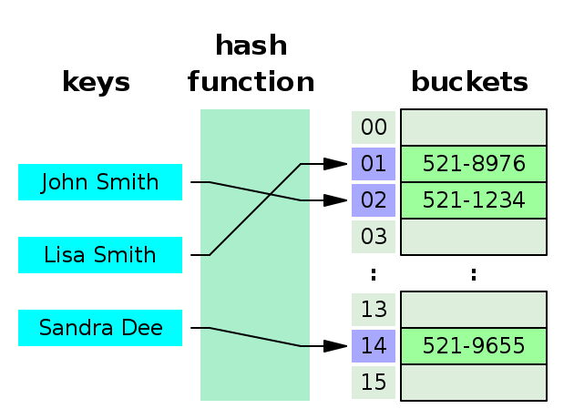
Figure 1 is a refresher of how hash tables works. Looking after a phone number in an agenda is a repetitive task, and we want it to be as fast as possible.

1. Hash collisions
Java maps and python dictionaries implementations differs from each other in how they solve hash collisions. A collision is when two keys share the same hash value. Hash collisions are inevitable, and two of the most common strategies of collision resolution are open addressing and separate chaining.
1.1. Separate chaining

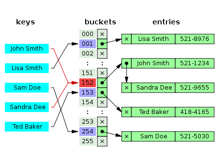
As shown in figure two, when two different keys point to the same cell value, the cell value contains a linked list with all the collisions. In this case the search average time is O(n) where n is the number of collisions. The worst case scenario is when the table has only one cell, then n is the length of your whole collection.
1.2. Open addressing
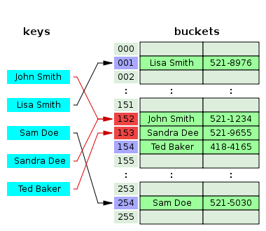
This technique is not as simple as separate chaining, but it should have a better performance. If a hash collision occurs, the table will be probed to move the record to a different cell that is empty. There are different probing techniques, for example in figure three the next cell position is used.

2. Java map
If we inspect the Hashmap class from the java.util package, we will see
that java uses separate chaining for solving hash clashes. Java also adds
a performance improvement, instead of using linked list to chain the
collisions, when there are too many collisions the linked list is
converted into a binary tree reducing the search average time from O(n)
to O(log2 n).
The code below correspond to the putVal method from the Hashmap
class which is in
charge of writing into the hash table. Line 6 writes into an empty
cell, line 17 inserts a new collision into a linked list and line 13
into a binary tree. Finally, line 19 converts the linked list into a
binary tree.
 1: final V putVal(int hash, K key, V value, boolean onlyIfAbsent, boolean evict) {
 2:     Node<K,V>[] tab; Node<K,V> p; int n, i;
 3:     if ((tab = table) == null || (n = tab.length) == 0)
 4:         n = (tab = resize()).length;
 5:     if ((p = tab[i = (n - 1) & hash]) == null)
 6:         tab[i] = newNode(hash, key, value, null);
 7:     else {
 8:         Node<K,V> e; K k;
 9:         if (p.hash == hash &&
10:             ((k = p.key) == key || (key != null && key.equals(k))))
11:             e = p;
12:         else if (p instanceof TreeNode)
13:             e = ((TreeNode<K,V>)p).putTreeVal(this, tab, hash, key, value);
14:         else {
15:             for (int binCount = 0; ; ++binCount) {
16:                 if ((e = p.next) == null) {
17:                     p.next = newNode(hash, key, value, null);
18:                     if (binCount >= TREEIFY_THRESHOLD - 1) // -1 for 1st
19:                         treeifyBin(tab, hash);
20:                     break;
21:                 }
22:                 if (e.hash == hash &&
23:                     ((k = e.key) == key || (key != null && key.equals(k))))
24:                     break;
25:                 p = e;
26:             }
27:         }
28:     }
29: }
The above code is extracted from the Java SE 17 (LTS) version, the binary tree improvement has been introduced in Java 8, in older versions the chaining was done only with linked lists.
3. Python dictionary
Python in contrast to java uses open addressing to resolve hash collisions. I recommend you to read the documentation from the source code: https://github.com/python/cpython/blob/3.11/Objects/dictobject.c Where the collision resolution is nicely explained at the beginning of the file.
Python resolves hash table collisions applying the formula
idx = (5 * idx + 1) % size, where idx is the table position.
Let's see an example:

- Given a table of size
8 - We want to insert an element in position
0, which is not empty. - Applying the formula, the next cell to check is position
1[(5*0 + 1) % 8 = 1] - The cell is not empty, next try is position
6[(5*1 + 1) % 8 = 6] - The following try is position
7 [(5*6 + 1) % 8 = 7] - Next try is position
4 [(5*7 + 1) % 8 = 5] - Etc…
Can you spot the pattern?
Python adds some randomness to the process adding a perturb value which is
calculated with the low bits of the hash, the final formula is
idx = ((5 * idx) + 1 + perturb) % size.
Unfortunately, the C source code of CPython dictionaries is not as straight
forward as Java code is. This is due to some optimizations that we will
see later on, when we will talk about performance. We can see the formula
idx = ((5 * idx) + 1 + perturb) % size
in action in the method lookdict_index, where line 9 is an infinite
loop to find out the index, line 17 recalculates the perturb value and
line 18 applies the formula.
 1: /* Search index of hash table from offset of entry table */
 2: static Py_ssize_t
 3: lookdict_index(PyDictKeysObject *k, Py_hash_t hash, Py_ssize_t index)
 4: {
 5:     size_t mask = DK_MASK(k);
 6:     size_t perturb = (size_t)hash;
 7:     size_t i = (size_t)hash & mask;
 8:
 9:     for (;;) {
10:         Py_ssize_t ix = dictkeys_get_index(k, i);
11:         if (ix == index) {
12:             return i;
13:         }
14:         if (ix == DKIX_EMPTY) {
15:             return DKIX_EMPTY;
16:         }
17:         perturb >>= PERTURB_SHIFT;
18:         i = mask & (i*5 + perturb + 1);
19:     }
20:     Py_UNREACHABLE();
21: }
4. Performance

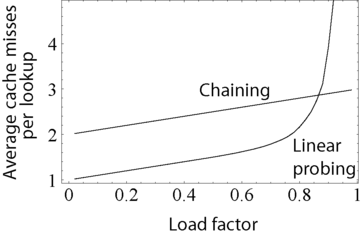
The above graph compares the average number of CPU cache misses required to look up elements in large hash tables with chaining and linear probing. Linear probing performs better due to better locality of reference, though as the table gets full, its performance degrades drastically.
Python uses dicts internally when it creates objects, functions, import modules, etc… Therefore, the performance of dictionaries is critical and linear probing is the way to go for them. The code below shows how python uses dictionaries internally when creating classes.
class Foo():
    def bar(x):
        return x+1

>>> print(Foo.__dict__)
{
  '__module__': '__main__',
  'bar': <function Foo.bar at 0x100d6b370>,
  '__dict__': <attribute '__dict__' of 'Foo' objects>,
  '__weakref__': <attribute '__weakref__' of 'Foo' objects>,
  '__doc__': None
}
4.1. Load factor
As we have seen the load factor is crucial for the performance of hash table, python has a load factor of 2/3 and java of 0.75. This makes sense, as linear probing performance is very bad when there are no empty hash spaces. On the other hand, java uses a threshold of 8 elements to switch from a linked list to a binary tree, as we can see in the code below.
static final float DEFAULT_LOAD_FACTOR = 0.75f;

/**
 * The bin count threshold for using a tree rather than list for a
 * bin. Bins are converted to trees when adding an element to a
 * bin with at least this many nodes. The value must be greater
 * than 2 and should be at least 8 to mesh with assumptions in
 * tree removal about conversion back to plain bins upon
 * shrinkage.
*/
static final int TREEIFY_THRESHOLD = 8;
5. What about sets
Dictionaries and maps are closely related to sets. In fact, sets are just dictionaries/maps without values. Indeed, Java uses this approach to implement sets, lets look at the source code:
/**
 * Constructs a new, empty set; the backing {@code HashMap} instance has
 * default initial capacity (16) and load factor (0.75).
 */
public HashSet() {
    map = new HashMap<>();
}
There are two different reasons why python does not reuse Objects/dictobject.c for implementing sets, the first one is that CPython does not use sets internally and the requirements are different. Looking after performance, CPython optimize the sets for the use case of membership. It is well documented in the source code to be found in Objects/setobject.c.:
/*
   Use cases for sets differ considerably from dictionaries where looked-up
   keys are more likely to be present.  In contrast, sets are primarily
   about membership testing where the presence of an element is not known in
   advance.  Accordingly, the set implementation needs to optimize for both
   the found and not-found case.
*/
A set is a different object and the hash table works a bit different, the set load factor is 60% instead of 66.6%, every time the table grows it uses a factor of 4 instead of 2, and the main difference is in the linear probing algorithm, where it inspects more than one cell for every probe.
6. Summary
CPython and Java use different approach to resolve hash collisions, while Java uses separate chaining, CPython uses linear probing. Java implements sets reusing hash tables but with dummy values, while python using also linear probing, optimizes the sets for different use cases, implementing a new linear probing algorithm. The reason for that is because CPython uses dictionaries internally and a high performance is critical for a proper performance of Python.
7. A note on source code
The source code examples are extracted respectively from the Java SE 17 (LTS) and CPython 3.11 versions.
